By Nikhil Vinod - April 28, 2026
Summary
Recently, I created a game on my personal website (this one!). My goal was threefold: gain thorough experience with Codex, make an interesting game concept, and gather player data for analysis. Throughout this paper, I analyze the EV of the different power-ups, the maximum possible score, and ideal choices for different game goals. In the future, I aim to analyze the collected data and compare it to the conclusions in this paper to verify its validity.
Introduction
My initial goal for this game was to make something that could collect player behavior data. I could have made any game, but I had an idea like this for a while. The game itself is primarily in TypeScript, hosted on my website. I used ChatGPT 5.4 in Codex to code the game. My main observation from using Codex is that it's great at creating logical structures and future-proofing, though quite bad at visual elements and design. However, I didn't intend to make it visually complex, so this wasn't an issue.

Figure 1: Screenshot of the initial game screen
I started by constructing simpler structures. Instead of making the full game from scratch, I aimed to take the most essential elements and build on top of them. My creation path was the following:
- Cup under the ball mechanism
- Wager component and victory component
- Power-ups last
- Other minor additions (leaderboard, music, etc.)
I kept the game as visually simple as possible to make it easy to understand. I also made sure it was optimized for mobile, as I believe most people prefer to access content on mobile devices.
The classic shuffling cups and ball game made this easy to accomplish. Traditionally, the game is skill-based, where a player tracks an item beneath shuffling cups. However, I felt that would be quite uninteresting and redundant. I was more inspired by a magician's sleight of hand when designing the game, as it creates a perception of randomness. Even when underlying probabilities are fixed, individuals often misinterpret randomness in decision-making contexts (Kahneman & Tversky, 1979). I used that randomness as the main premise.

Figure 2: Example of the game where a ball is shuffled by cups
To add strategy and player investment, I added a wagering component, where each player must bet a minimum number of coins. Interactive decision-making elements and reward systems help increase engagement and perceived agency in the game (Koster, 2013; Salen & Zimmerman, 2004). For my data gathering purposes, this adds a lot of behavioral information. It also allows the player to have more diverse playstyles. In order to add elements of skill, I added power-ups to assist with the player's wagering decisions.
There are currently 8 power-ups in the game. My design principle was to make interesting power-ups. I started by incorporating easy power-ups that modify win odds and win return. I then decided to incorporate more interesting ideas based on classic psychology and game theory concepts, including Monty Hall and Prisoner's Dilemma. All my power-ups are discussed extensively in the EV calculation section.
Standard victory conditions involve getting to 200 points by the end of round 10. Additionally, the top ten highest scores among all players at the end of round 10 are placed on a global leaderboard. I created this to increase the incentive for playing the game. To further this goal, I intend to add more power-ups and game modes.
There is no real consistent visual theme currently. I aim to create an artwork for each power-up as well as music options. However, this action is not particularly relevant to my main goal of data collection.
Regarding that, every round, player's choice information is stored in a SQL table in Supabase. The player is saved across turns and games, stored locally in their history. If a player clears their browser history, they will be seen as a new player. However, I believe this won't be an issue for my purposes. My goals with the data include the following:
- Compare the player data with the expected data.
- Account for the fact that human decision-making frequently deviates from rational models due to cognitive biases (Kahneman, 2011).
- Understand how players' behavior responds to different power-ups and results.
- Identify what changes I can make to balance the game or make it more interesting.
I'll go into further detail regarding the data in the next report.
From here on, I am presenting the expected value (EV) calculations and breakeven points for game mechanics.
Some important notes:
- Starting coins are 100.
- The requirement to win is 200 by or before the end of round 10.
- The minimum wager is 10 coins, or all remaining coins if you do not have 10.
- A player loses if their coin value becomes 0 or less.
- Players can only choose one power-up per shop and must pay whatever price is associated with the power-up using their coins.
- Power-ups cannot appear in a shop after one has already appeared and been chosen.
EV Calculations
Basic EV Formula
EV = P(Win) * (Win Multiplier * I) + P(Lose) * L - I - Price
Where:
I= initial wagerL= loss returnPriceapplies only when using power-ups
No Power-Up Standard Run
Win return:
EV = (1/3)(2 * 10) + (2/3)(0) - 10 = -10/3 ~= -3.33
The standard expected return per turn is losing 3.3333 coins. Assuming I is the only independent variable, we can take the derivative of the above equation. Doing so, we receive a value of -0.33. Therefore, the expected return will only become more negative as I increases, making breakeven impossible.
If no power-ups are taken, the average number of coins the player is expected to have at the end of round 10 is:
Final = 100 + (-3.33 * 10) ~= 66.67
On average, the player is expected to lose for the standard wager. Since the EV always remains negative, any greater wagers have the same result.
Assuming constant victory, higher wagers result in higher returns. The smallest amount bet, the enforced minimum, is 10. Consequently, the gain can only be 10 through standard play. This means it would take 10 turns to win with constant victory and minimum bets. Victory in any one round is 1/3, so victory over ten turns is:
PMinBetWin = (1/3)^10 = 0.0017%
The general victory equation can be represented by the following:
PBet_Win = (1/3)^(100 / w)
Where w is the constant amount wagered per turn. The exponent in the equation is the requirement to win divided by the win multiplier and wager, which reduces to 100 / w. We see that the limit as w approaches infinity causes the probability of winning to approach 1, under idealized assumptions, reflecting standard asymptotic behavior in probabilistic models (Feller, 1968). Technically, any wager at or over 200 means that the player has already won. Therefore, this equation is bound (10, 200).
We see from the equation that to win as fast as possible, and with the best odds, a player must wager as much as possible. This results in the player betting their full starting coins for a 33% chance of winning on the first turn. With no other information, the best strategy is to wager everything and play the game repetitively until you win. From a purely EV standpoint, the optimal strategy is to wager the maximum possible amount, as risk-neutral models favor maximizing potential returns (Epstein, 2013); however, behavioral research suggests that real players are typically loss-averse and unlikely to follow such strategies consistently (Kahneman & Tversky, 1979), at least without proper incentive.
In order to prevent this brainless excursion, I created the concept of "power-ups."
Power-Up EVs
Halve EV
Halve is a power-up that decreases your wager loss in the next round. The player only loses half of their wager if they choose this power-up during a losing round, and they receive the other half back. From here, we return to the former equation:
EV = P(Win) * (Win Multiplier * I) + P(Lose) * L - I - Price
EV = (1/3)(2I) + (2/3)(1/2I) - I - 3
And if I = 10, the minimum wager value:
EV = -3
In fact, regardless of the initial wager, the EV will always be -3. All the terms except for the price cancel. From an EV standpoint, since the EV of this power-up is greater than the standard, the player is mathematically favored to choose Halve over choosing nothing. Nevertheless, real-world decision-making may differ due to risk aversion (Kahneman & Tversky, 1979).
The player is expected to end with 69.67 coins with conservative wagering over 10 rounds if Halve is used every round except the first. If we consider the fact it can only be used 5 times max in a game, we get 68.33 instead, a minute difference. Regardless, we see taking Halve is worth long-term over not taking it at all. Since it has a constant EV and standard betting has worsened EV over time, it becomes better to take Halve if the wager gets higher.
An additional note is this does not affect the victory equation from prior. Since the player now has an additional cost, it increases the number of wins required. Nevertheless, as previously discussed, the best strategy is to wager high, which we know benefits from Halve. From this, we see Halve as a strong defensive option.
Quadruple EV
Quadruple takes your wager and 4x it for the win with standard loss outcomes. The calculations for this are similar to Halve:
EV = (1/3)(4I) - I - 5
And adding the minimum wager in:
EV = -1.67
This is the best EV yet, although still not positive. However, we can see the derivative of the EV equation is a positive value in this instance, 0.333, unlike before. The EV will be positive with a high enough wager.
Calculating breakeven, we get the following:
I > 15
The higher the wager, the higher the EV for Quadruple.
Hedge
Hedge takes your wager and reverses the odds for a lower payout. Win odds increase to 2/3, but payout lowers to 1.5x from 2x. The calculations are the following:
EV = (2/3)(3/2I) - I - 5
And adding the minimum wager in:
EV = -5
Calculating breakeven, we get the following:
I > 50
The result is indeterminate. There is no value for the initial wager that results in a positive EV. In fact, the derivative of the EV equation is 0, the same as Halve. The EV will always be to lose 5 coins. However, since the standard bet is expected to lose more coins the higher the initial wager is, at any initial wager greater than 15, it is more favorable to choose Hedge than standard.
From a pure EV perspective, Hedge seems worse than Halve.
PlusTwo
PlusTwo adds two more balls with variant outcomes. The green ball has 3x wager, white is 1.5x wager, and red is an extra loss of 1 wager. The calculations are the following:
EV = (1/3)(3I) + (1/3)(3/2I) + (1/3)(-I) - I - 7
EV = (1/6)I - 7
And adding the minimum wager in:
EV = -32/6 = -5.33
Calculating breakeven, we get the following:
I > 42
The derivative of the EV is positive, so the EV gets higher the higher the initial wager is. When the player wagers over 42, they will be expected to make a positive return on average.
Monty
Monty is the classic Monty Hall problem. After the first choice, one wrong cup is removed, and the player gets the option to switch. This results in the following odds of getting it right: 2/3 chance to choose wrong and a 1/3 chance to choose right.
If the wrong one is chosen, the other non-chosen cup that wasn't removed is guaranteed to be the winning cup, while the opposite is true if the player chose right the first time. This means the optimal decision is to always switch (vos Savant, 1990). Therefore, the EV becomes the following:
EV = P(Win) * Win_Multiplier * Initial_Wager + P(Lose) * Lose Return - Initial Wager - Price
EV = (2/3) * 2 * I + (1/3) * 0 - I - 10
EV = (1/3)I - 10
And adding the minimum wager in:
EV = -20/3 = -6.67
Calculating breakeven, we get the following:
I > 30
Prisoner's Dilemma
The Prisoner's Dilemma power-up is the classic Prisoner's Dilemma, where the player can choose to either betray or cooperate with the prisoner, a foundational concept in game theory used to analyze cooperation and competition (Axelrod, 1984). Like the standard Prisoner's Dilemma, the best outcomes come from betraying the prisoner rather than cooperating.
The player gets 3x their wager if they choose to betray and the prisoner cooperates, while they get 1.5x their wager if both betray. The player gets 2x if both cooperate, and gets nothing if the player cooperates and the prisoner betrays.
Currently, the prisoner has a 2/3 chance of cooperating and a 1/3 chance of betraying. However, the more the player betrays, the higher the chances of the prisoner betraying. Additionally, the more the player cooperates, the more the prisoner cooperates. These do have limits in place that are not 0% or 100%.
EV for first betray:
EV = (13/12)I - 10
And adding the minimum wager in:
EV = 10/12 = 0.833
Calculating breakeven, we get the following:
I > 9.23
Therefore, the EV is almost always positive for choosing Betray and gets greater the more is wagered for the first Prisoner's Dilemma use.
EV for first cooperate:
EV = (1/3)I - 10
And adding the minimum wager in:
EV = -20/3 = -6.67
Calculating breakeven, we get the following:
I > 30
The EV is positive for any wager greater than 30 coins. For a maxed-out Prisoner's Dilemma, the odds change and thus have the following results.
EV for maxed betray:
EV = -0.7225I - 10
And adding the minimum wager in:
EV = -17.225
Calculating breakeven, we get the following:
I < -13.842
Here, we notice the EV is no longer always positive. Furthermore, it is impossible for the player to get a positive EV, as they must bet less than a negative value, which is impossible.
EV for maxed cooperate:
EV = (3/5)I - 10
And adding the minimum wager in:
EV = -4
Calculating breakeven, we get the following:
I > 16.67
The EV is positive for any wager greater than 16.67 coins. Notice this is lower than the breakeven for the first cooperation. Furthermore, this shows that in iterated form, it is more ideal to cooperate in comparison to betrayal. This mirrors findings from the iterated model of the original Prisoner's Dilemma, where cooperative strategies often emerge as optimal over repeated interactions (Axelrod, 1984).
An additional note is that the first choice of cooperation already maxes out the cooperation chance in the next Prisoner's Dilemma. However, the betray option takes two selections before maxing out the prisoner bias.
Therefore, we obtain a mid-betray option EV:
EV = 0.185I - 10
And adding the minimum wager in:
EV = -8.15
Calculating breakeven, we get the following:
I > 54.05
This indicates that it still may be slightly optimal to choose to betray twice if the values wagered are high enough. However, future wagers for Prisoner's Dilemma will be heavily affected. Another point to note is that trying to switch to cooperation after two rounds of betrayal will, on average, result in a total wager loss, making the round a wasted opportunity. This reduces tempo, with a high chance of a minimum 10-point loss.
Marshmallow
Marshmallow is based on the Stanford marshmallow experiment conducted by Dr. Walter Mischel to study delayed gratification and self-control in decision-making (Mischel et al., 1972). The player can choose to immediately receive 10 coins or wait for an undetermined number of rounds to receive 30 coins in the near future. The numbers were adjusted for balancing purposes, not exactly double, as stated in the original experiment. I also added a variable time for the reward payout with a small percent chance of no reward. I did this to represent the lack of trust in whether the reward payout would occur. This uncertainty in reward timing reflects later findings that delayed gratification behavior is influenced by environmental reliability and trust, rather than purely self-control (Watts et al., 2018).
EV calculations:
Now:   10 + EV standard roll = 6.67
Later: 30 + EV standard roll = 26.67
As the initial wager increases, the expected return gets lower for both instances. Therefore, it's better to wager less after choosing Marshmallow on average. For the delayed choice, the expected turn received is 2 with a small chance of never, so slightly over 2, the EV is for every 2 turns.
Invest
The Invest power-up has a mechanism quite unlike any of the other power-ups. For one, it requires two shop uses to utilize fully. The Invest power-up works via the following mechanism: the player can choose to invest coins they own up to the coins they have minus 1. The invested coins will grow by 10% compounded every round, where returns increase exponentially over time, a fundamental principle in financial theory (Graham, 2006). The invested coins are non-liquid and do not count towards the final score unless taken out. When the Invest power-up reappears in the shop, the coins can be taken out, which counts as a second power-up purchase. The latest this purchase can occur is after round 9, the final shop. The Invest option also does not appear guaranteed in the shop and has the same chance of spawning as any other power-up.
Ideal gameplay with Invest would be the following: invest as much as possible into Invest and let it grow, then wager as little as possible to maintain survival. The minimum bet is 10 coins to counter this.
Suppose the following scenario. The player wagers 10 in round 1 and loses it. They then invest 80 of their remaining 90 in the shop. In round 2, they must wager their last 10. There is a 2/3 chance they immediately lose, and a 1/3 chance they continue. These are standard odds. Therefore, the player is expected to lose 3.33 per turn. With this in mind, the player needs 3.33 per turn for 9 turns, or 30 coins. In the scenario where the player loses the first round, they could, on average, safely invest 60. Growth by round 9 would be:
F = P * 1.1^8
60 * 1.1^8 = 128.6
If the player wins the first round and invests their coins up to an amount where they still keep 30, growth by round 9 would be:
80 * 1.1^8 = 171.487
In either of these most conservative scenarios, it would be expected, on average, the player would fail to win by only using Invest, assuming they can pull out on round 9. However, in combination with other power-ups, victory becomes more likely as the player can grow enough to cover the excess that Invest cannot provide. The player can also invest greater amounts during later turns for higher returns, though that is dependent on victories before the investment.
I developed an equation to determine the growth of coins while incorporating the dependency on the minimum round requirement:
Investment payout = (c - 10n)(1.1)^n
Where c is the number of coins the player has, and n is the number of rounds the coins are invested in. n is limited by the max number of rounds minus two, one for investing and one for taking out. c as a value can get higher as the round number increases, but that means n will have a lower ceiling. The 10 is subtracted because that is the minimum amount necessary for a bet. However, future turns would be affected, so 10 must be chosen.
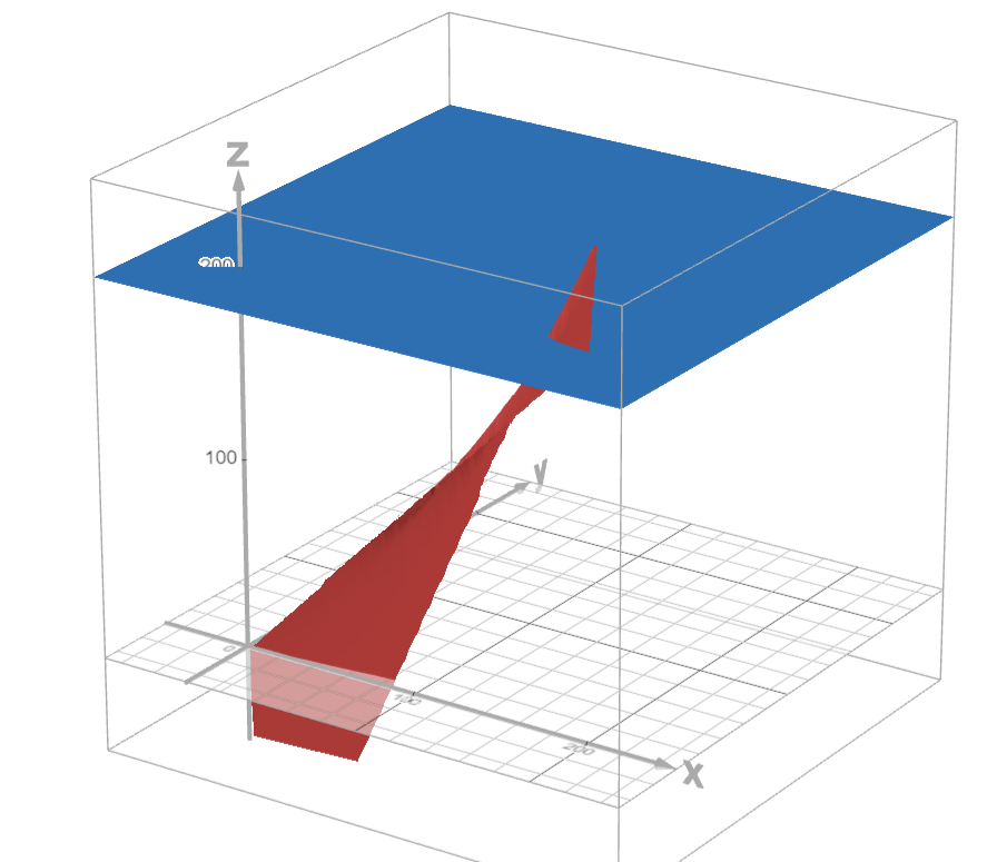
Figure 3.1: Three-dimensional graphical representation of the investment payout via Desmos
In the above graphical representation of the equation, x is c, y is n, and z is the investment payout. The red figure is the equation, and the blue plane is the win requirement of 200. The graph constrains y from 0 to 8, as the number of rounds the coins are invested for cannot exceed that. Additionally, the input coins have a floor of 0 due to being unable to invest negative amounts. I also added a ceiling of 200 as the game would've already been won at that point.
For the final invested amount to be 200 or greater, I set z to 200 and graphed the resulting equation with the same constraints. This graph gives the set of values of both c and n that allow for victory from Invest.
200 / 1.1^n + 10n < c
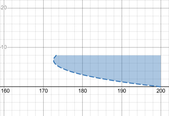
Figure 3.2: Graphical representation of breakeven values for Invest via Desmos
One final concept to consider for Invest is the breakeven. Since there are two variable terms in using Invest, there is no one breakeven value, but an equation. Since using Invest uses up two shop uses, the cost is just the EV of two standard rounds: -20/3. The EV equation becomes:
EV = c(1.1)^n - c - 20/3
Then adding in 0 and solving for n, we get the following solution for breakeven:
n > log_1.1((20 / 3c) - 1)
Theoretical Limits
The domain of a player's coin values at the end of round 1 fit within [0, 200]. The theoretical maximum at the end of round 10 requires the following outcomes. The first round must be a standard win with all starting coins wagered. Then, the greatest possible return is through Quadruple. However, because no power-up can be bought in successive shops, the most that can be bought in a standard run is 5 times. This accounts for 6 of the rounds. The next highest return is 3x. This can occur either through Prisoner's Dilemma or PlusTwo. Using these values, we can obtain the overall multiplier, assuming a win every turn:
MultMax = MultStandard * MultQuadruple^5 * MultPlusTwo^4
MultMax = 2 * 4^5 * 3^4 = 165,888
Multiplying with the starting coins, we receive a maximum possible number of coins: 16,588,800.
An additional note is the cost of the power-ups to find the actual final score. Since 5 Quadruple uses 5 coins and 4 PlusTwo uses 7, a player would spend 53 coins. Subtracting that from the total, I obtained 16,588,747 maximum coins.
The main issue with this solution for including price is that it does not include gameplay. In reality, the price is subtracted before a multiplier the next round. Due to this, the price cannot simply be subtracted at the end. Following the ideal route, the actual maximum score ends up being: 15,978,040 coins.
However, it's important to consider how unlikely such a scenario is. To start, winning the first cup is already a 1/3 chance. The same continues to be true for Quadruple. Since Prisoner's Dilemma gets harder, the better choice for odds would be PlusTwo, also 1/3. With this, we simply get:
OddsBaseMax = (1/3)^10 = 0.00169%
Now this may seem high, but it's important to remember the shop odds are not guaranteed and need to be a very precise spawning. Since the first shop has no shop restrictions, we want the following:
PSpawnQuadruple = 1 - ((n - r) / n)
PSpawnQuadruple = 1 - ((8 - 3) / 8) = 3/8 = 37.5%
In all future shops, since the previous shop item cannot spawn, the odds increase slightly:
PSpawnDesired = 1 - ((n - r - 1) / (n - 1)) = 3/7 = 42.857%
So for all the shops to spawn exactly as intended, it must be:
PSpawnIdeal = (3/8) * (3/7)^8 = 0.01676%
Combining this ideal shop spawn with the ideal selection spawn for the theoretical maximum score, we obtain the following probability of such a score:
PScoreMaximum = (1/3)^10 * (3/8) * (3/7)^8
PScoreMaximum = 0.0000000028383164179 = 2.84 * 10^-7%
Although it is low, it remains theoretically possible within a probabilistic framework (Blitzstein & Hwang, 2019). If every American were to play this game once, there's a slightly over 60% probability that at least one person in the country would win due to the law of large numbers (Feller, 1968).
Another hypothetical can be built in the following way. The record for winning in round one is slightly over 4 seconds. Adding on some buffer and shop time, I estimate 15 seconds per round. Current preliminary estimates of some runs seem to have a similar value as well. Assuming the player restarts immediately if unsatisfactory to the max record, we can represent this with the following series:
sum from n = 1 to 10 of 10 * n * (1/3)^(n - 1)
This accounts for the probability of choosing the right cup. However, the player choosing to restart the game is also dependent on the shop outcome. This causes the following changes:
13 * 5/8 + sum from n = 2 to 10 of (165/28) * n * (10/21)^(n - 2)
= 49.434 seconds
This equation is the weighted average of the expected game times. Note that the round ten success rate was not included because its effect would be negligible. In fact, since wins and losses are essentially the same length for all rounds, this decision is validated.
What this estimated time tells us is the following: an individual who plays to achieve the best score most optimally can spend 2/3 of every day playing the game and will still have only a 26.5% chance of winning over a 100-year period.
Optimal Strategy
Optimal strategy takes two different routes for this game, known as utility theory, where different players optimize for different outcomes based on their risk preferences and goals (Knight, 1921). A player can either optimize to increase the chance of winning each game session or get the highest score possible. These two run counter to each other, as getting the highest score involves higher-risk, higher-reward actions, reducing the chance of victory in any given game session.
Game Winning
Winning this game means achieving at least 200 coins by round 10. For optimization's sake, this should be possible as often as possible. Using this metric, EV becomes an important tool. Not only that, but higher EVs at lower wager amounts become more important to reduce.
In order from best to worst, I've determined the following:
- Delayed Marshmallow
- Invest
- Marshmallow
- Prisoner's Dilemma Betray*
- Quadruple
- Halve
- Standard
- Hedge
- PlusTwo
- Prisoner's Dilemma Cooperate*
- Monty
The Prisoner's Dilemma options are ranked concerning the first selection.
Including the fact that if certain amounts of coins are wagered, EVs can increase, we see the following modified list instead:
- Delayed Marshmallow
- Invest
- Marshmallow
- Prisoner's Dilemma Betray
- Quadruple
- Prisoner's Dilemma Cooperate
- Monty
- Halve
- Standard
- Hedge
Due to the varying growth factors, certain power-ups will be more optimal at varying wagers. This can be deduced from the earlier EV equations presented.
High Scoring
As mentioned earlier, making a high-scoring run is more about high-risk, high-reward options. Nevertheless, winning as often as possible is important with as much on the line as possible. Due to this, high odds with an increasing multiplier become more important.
The following list was constructed with this in mind. Since everything's on the line anyway, a loss is game-ending. To reduce this, winning odds being the highest possible is relevant. Some guaranteed EV options are also much less valuable since they guarantee so fewer coins than could be achieved in other ways. With that in mind, the list is the following:
- Prisoner's Dilemma Cooperate
- PlusTwo
- Monty
- Hedge
- Quadruple
- Prisoner's Dilemma Betray
- Halve
- Marshmallow
- Delayed Marshmallow
- Standard
- Invest
The Betray option for Prisoner's Dilemma is a good option the first time it's used. Successive uses make it much weaker. Since the list is for overall selections, it's been pushed down in the rankings for that reason. It also directly prevents the usage of the best option, so it takes that into account as well. An interesting observation is how many of the power-ups at the bottom of the first list are rearranged closer to the top of this list.
Conclusions
Different game goals result in different ideal power-up choices. By using EV values for power-up outcomes and win rate odds, I constructed a list of what I believe are the best choices for each play style. Playing to win focuses on EV to increase the guarantee of a win and prioritizes power-ups with more certain outcomes. Playing for a high score focuses on the maximum odds of winning, in a high-risk, high-reward focus.
Currently, these are the expected ideal choices for each playstyle. In order to confirm this, I will be analyzing player data and comparing it to my predictions in a future paper. I'll also be using the data to determine balancing and new game modes or power-ups I can add in.
Ultimately, my goal is to practice game theory and quantitative analysis. By practicing and building this game, I aim to build a foundation to be applied to other fields. My goal is to analyze financial and business markets in the future and practice skills in concert with them.
-- Nikhil
References
- Axelrod, R. (1984). The evolution of cooperation. Basic Books.
- Blitzstein, J. K., & Hwang, J. (2019). Introduction to probability (2nd ed.). Chapman & Hall/CRC.
- Epstein, R. A. (2013). The theory of gambling and statistical logic (2nd ed.). Academic Press.
- Feller, W. (1968). An introduction to probability theory and its applications (Vol. 1, 3rd ed.). Wiley.
- Graham, B. (2006). The intelligent investor (Rev. ed.). Harper Business.
- Hull, J. C. (2018). Options, futures, and other derivatives (10th ed.). Pearson.
- Kahneman, D. (2011). Thinking, fast and slow. Farrar, Straus and Giroux.
- Kahneman, D., & Tversky, A. (1979). Prospect theory: An analysis of decision under risk. Econometrica, 47(2), 263-291.
- Knight, F. H. (1921). Risk, uncertainty and profit. Houghton Mifflin.
- Koster, R. (2013). A theory of fun for game design (2nd ed.). O'Reilly Media.
- Mischel, W., Ebbesen, E. B., & Raskoff Zeiss, A. (1972). Cognitive and attentional mechanisms in delay of gratification. Journal of Personality and Social Psychology, 21(2), 204-218.
- Salen, K., & Zimmerman, E. (2004). Rules of play: Game design fundamentals. MIT Press.
- vos Savant, M. (1990). Ask Marilyn. Parade Magazine.
- Watts, T. W., Duncan, G. J., & Quan, H. (2018). Revisiting the marshmallow test: A conceptual replication investigating links between early delay of gratification and later outcomes. Psychological Science, 29(7), 1159-1177.